Introduction

Diffuse gliomas are a rare kind of brain tumor. According to the National Institutes of Health, a piece of tumor tissue has to be surgically removed to get an accurate diagnosis. “Given their location within the brain, the live biopsy happens during surgery to confirm the presence of cancerous tissue,” says Solution Engineer Alejandro Morales Martinez, of HPE AI Solutions.

Alejandro has a PhD in biomedical engineering and extensive experience in deep learning techniques for clinical applications in medical imaging. “As with most types of cancer, early detection can lead to the best patient outcomes, especially in critical structures like the brain, where you’d have to remove sensitive healthy tissue to even get to it. MRI is uniquely suited to detect soft tissues within the brain and has the flexibility to distinguish between healthy brain tissue and gliomas.”

For rare tumors like these, a deep neural network trained specifically to recognize those tumors from MRI images could dramatically help in the early detection stage.

“The dataset [UCSF-PDGM: The University of California San Francisco Preoperative Diffuse Glioma MRI] was created as a research tool. In this dataset, we know that these are confirmed gliomas, and we have the actual imaging that goes with it, so it gives you a way to flag [cancer] ideally earlier on, while they are forming… so that eventually you can do more aggressive treatments to stop the cancer from spreading further.”

Alejandro and the solution engineering team at HPE work with a leading research hospital in the United States to provide deep-learning platforms and services to support clinical research on real-world data for MRI image segmentation as well as other use cases.

What is 3D structural segmentation? 

While many publicly available MRI datasets are 2D, UCSF-PDGM features predominantly 3D imaging. According to a study from the NIH comparing 2D, 2.5D, and 3D approaches to brain image segmentation, the 3D approach is more accurate, faster to train, faster to deploy, and shows better performance in the setting of limited training data: “Since the 3D approach provides more contextual information for each segmentation target, the complex shape of structures such as the hippocampus can be learned faster, and, as a result, the convergence of 3D models can become faster”.

Think of processing 3D data like a language modeling task: language models benefit from a longer context length, which increases the window of preceding and subsequent tokens around the predicted tokens. In the same way, the contextual information from the 3D shape for the 3D segmented structures produces smoother segmentation margins for structures of interest, when compared to a 2D segmentation model that treats each image independently. In addition, producing 3D segmentations is especially important when postprocessing the masks to extract radiomic features, or to perform downstream tasks like shape modeling.

💡Radiomic features are characteristics extracted from medical images, like CT scans or MRIs, using advanced software. These features capture details that might not be visible to the human eye. They include measurements such as the shape, size, texture, and intensity of the tissues shown in the images. By analyzing these features, doctors and researchers can learn more about a disease’s characteristics, like how aggressive a tumor might be, without needing invasive procedures. This can help in diagnosing diseases, predicting outcomes, and customizing treatment plans for patients.

What does the data look like?

In our demo, we use 87 of the 495 total subject data provided in the dataset. The dataset is formed by taking several MRI scans for each patient, “skull stripping” the scan (leaving just the brain image), and anonymizing the patient’s personally identifying information. The result is 4 MRI volumes per subject, as well as a target segmentation mask.

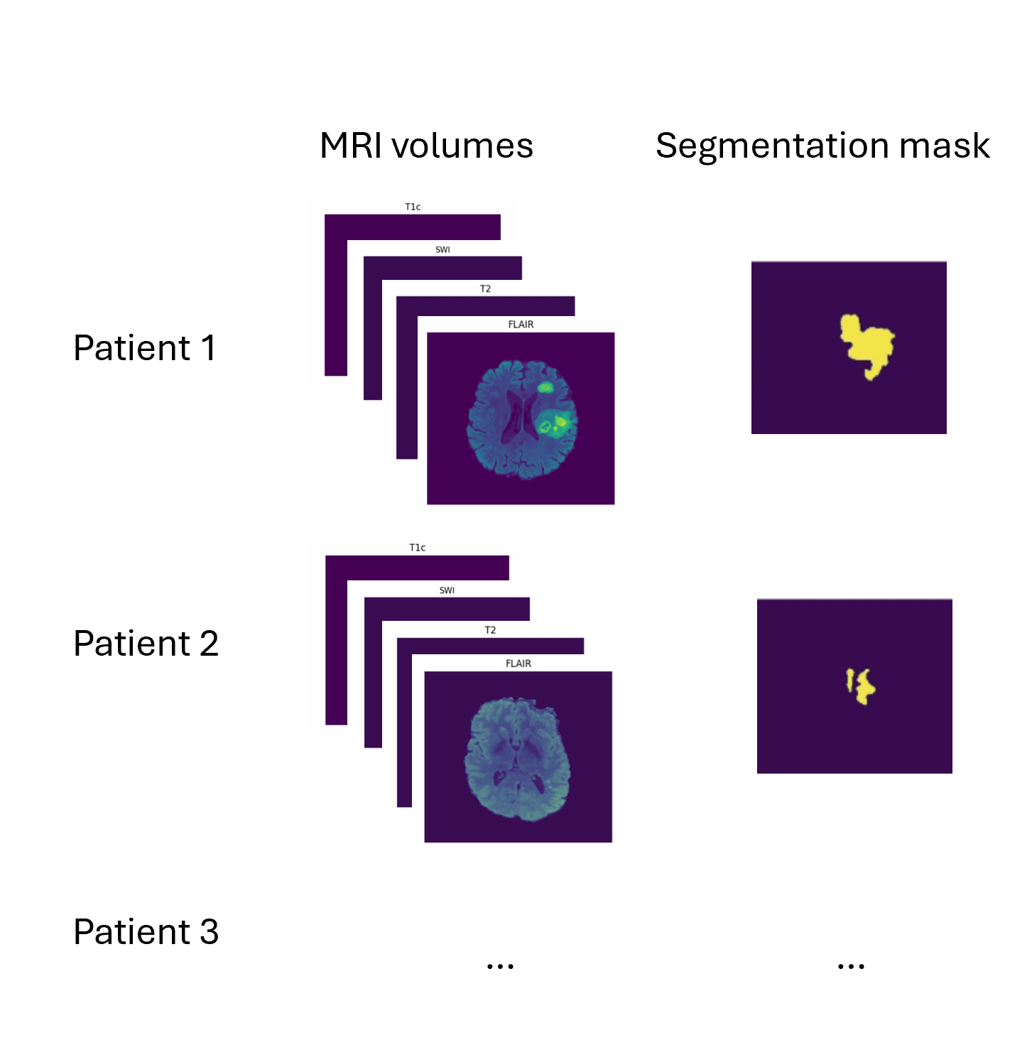
What is a 3D volume?

A volume is a collection of voxels - like a stack of images - that make up a 3D MRI scan. Each volume corresponds to a different type of scan that were each taken using different MRI frequency settings.

Some definitions: 

Voxel: a 3D pixel. Instead of having 2 coordinates, like for a pixel (x, y), you have 3 (x, y, and z) to define a voxel in 3D space. 

Mask: The voxels from the volume that are part of the tumor – the “ground truth”. In 2D computer vision, you define the right “pixels” as ground truth (like a car bounding box). Here, a 3D segmentation mask defines the right “voxels” as ground truth. 

Andy’s Brain Book has some great explanations of brain modeling specific terminology if you’re curious to learn more.

Demo Walkthrough

In our demo, all this data is stored and versioned in a Pachyderm repository, which acts like git for your data. In the data exploration stage of our project, we can connect to the Pachyderm repo via the Pachyderm Python SDK, and look at the files in the directory:

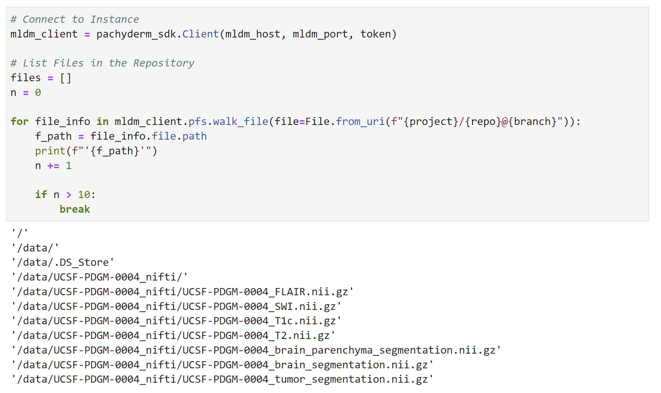
Notice how there are different MRI volumes, e.g., FLAIR, SWI, T2, etc., as well as segmentation masks: tumor_segmentation, etc., in each patient folder (for example, patient 0004).

To create a data frame such that each data point has a patient index, a set of MRI volumes, and the tumor segmentation mask, we can use Pandas:

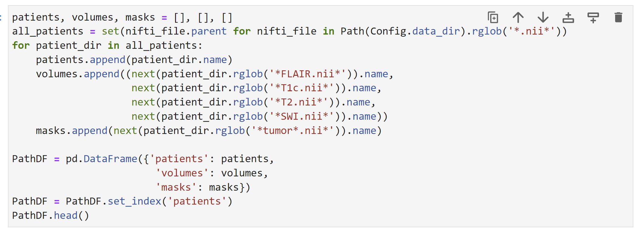
Here’s a snapshot of what the data looks like afterward:

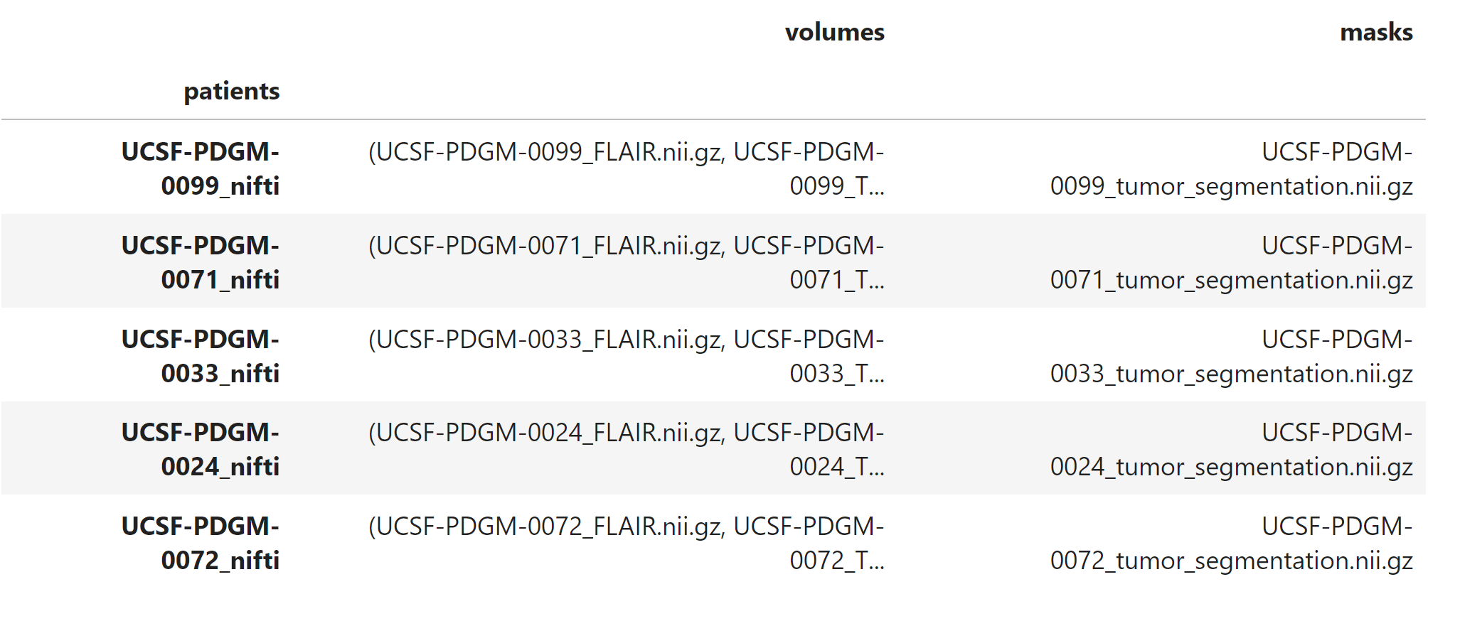
This preps and organizes the data so that it’s ready for model training (patient name, volumes (samples), masks (labels)).

Model Training

Since you can’t teach a regular 2D convolutional network to recognize 3D patterns, we’re going to use a special model called V-net. V-Net is designed to work with 3D image data, which is common in medical imaging (like CT scans and MRI images). Unlike its predecessor, the U-Net, which primarily handles 2D images, V-Net processes three-dimensional data directly. This allows it to better understand and interpret the spatial relationships and structures within the body, which are crucial for accurate segmentation. Check out V-net’s architecture:

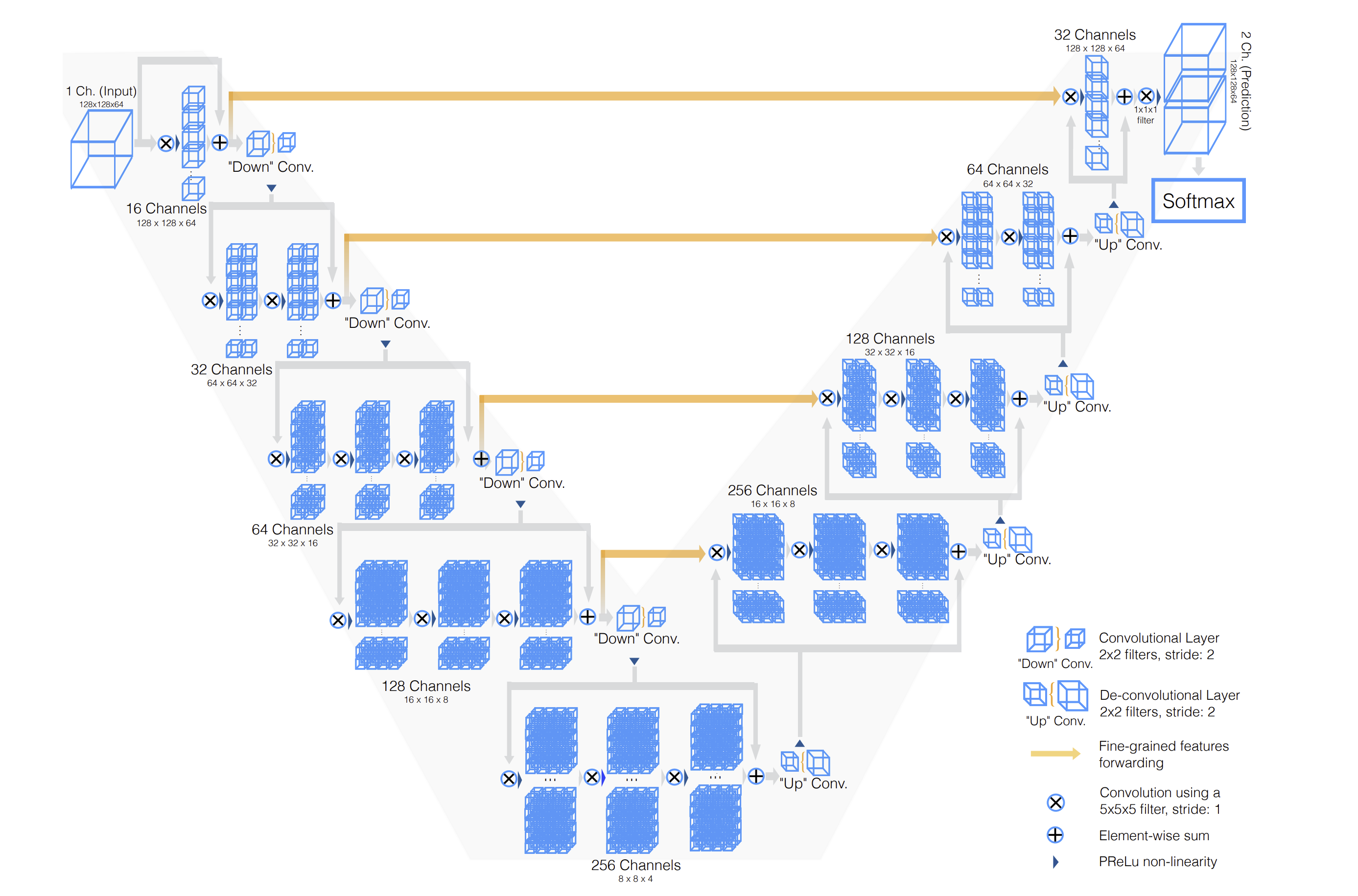
The architecture diagram shows an input with only a single channel, but it can be extended to any number of input channels, corresponding to the number of MRI volumes. V-net accepts 5D inputs, (batch, channel, depth, width, height) and outputs a 5D output (batch, one-hot predictions, depth, width, height). In our case, this dimension would be (batch, 4, 224, 224, 144) – corresponding to the 4 MRI volumes.

Changing the number of input channels also modifies the number of input convolution filters in the first convolution.

The architecture of the network is designed as an encoder-decoder setup:

• The encoder compresses the essential features needed for segmenting the image, while the decoder expands these features to recreate the detailed, labeled segmentation of the image.

• The architecture also incorporates skip connections, which are crucial for preserving details lost in the compression process. This prevents the model from overfitting, the gradients from vanishing, and helps the network learn faster.

Optimization

A commonly used optimization method in medical image segmentation is the Dice loss. Why is that?

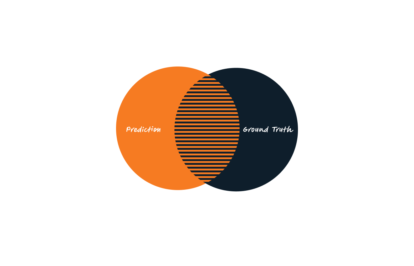
Dice coefficient is defined as the following: two times the intersection of the predicted and ground truth mask, divided by the total area of the ground truth and predicted mask. The Dice loss is simply (1 - Dice coefficient). The Dice coefficient is similar to the IOU metric, which is another popular metric used to optimize models on image segmentation tasks:

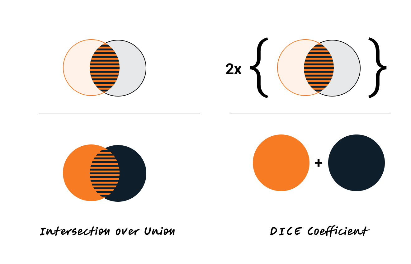
Dice loss is sometimes preferred for medical segmentation tasks over IOU (if only using one optimization criteria). By counting the intersection twice, it inherently values the correct predictions more heavily relative to the total size of both the prediction and the ground truth, which helps in cases with small target areas.

To train the model, we can simply train using standard PyTorch functions (documented in cells 11 to 16 of the Jupyter Notebook), or submit an experiment through Determined. Either way, we’re using the same code – the Determined experiments are just using PyTorchTrial to wrap the experiment code for ease of execution and advanced training and modeling capabilities Determined is well known for.

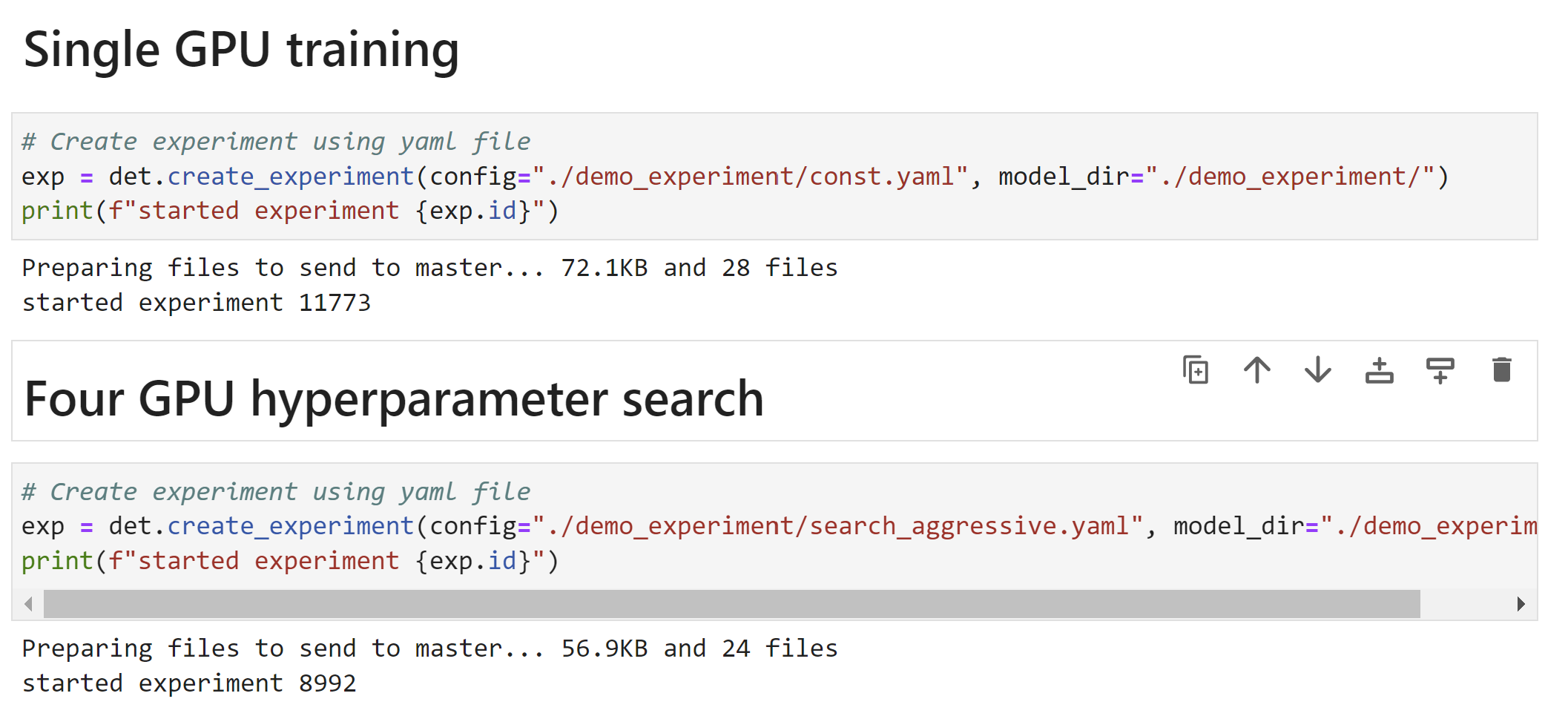
Once it’s done training, we can grab the best checkpoint from the experiment and use it to visualize some predictions:

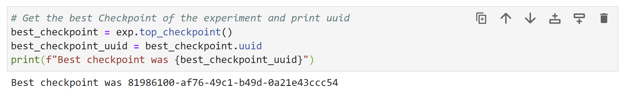
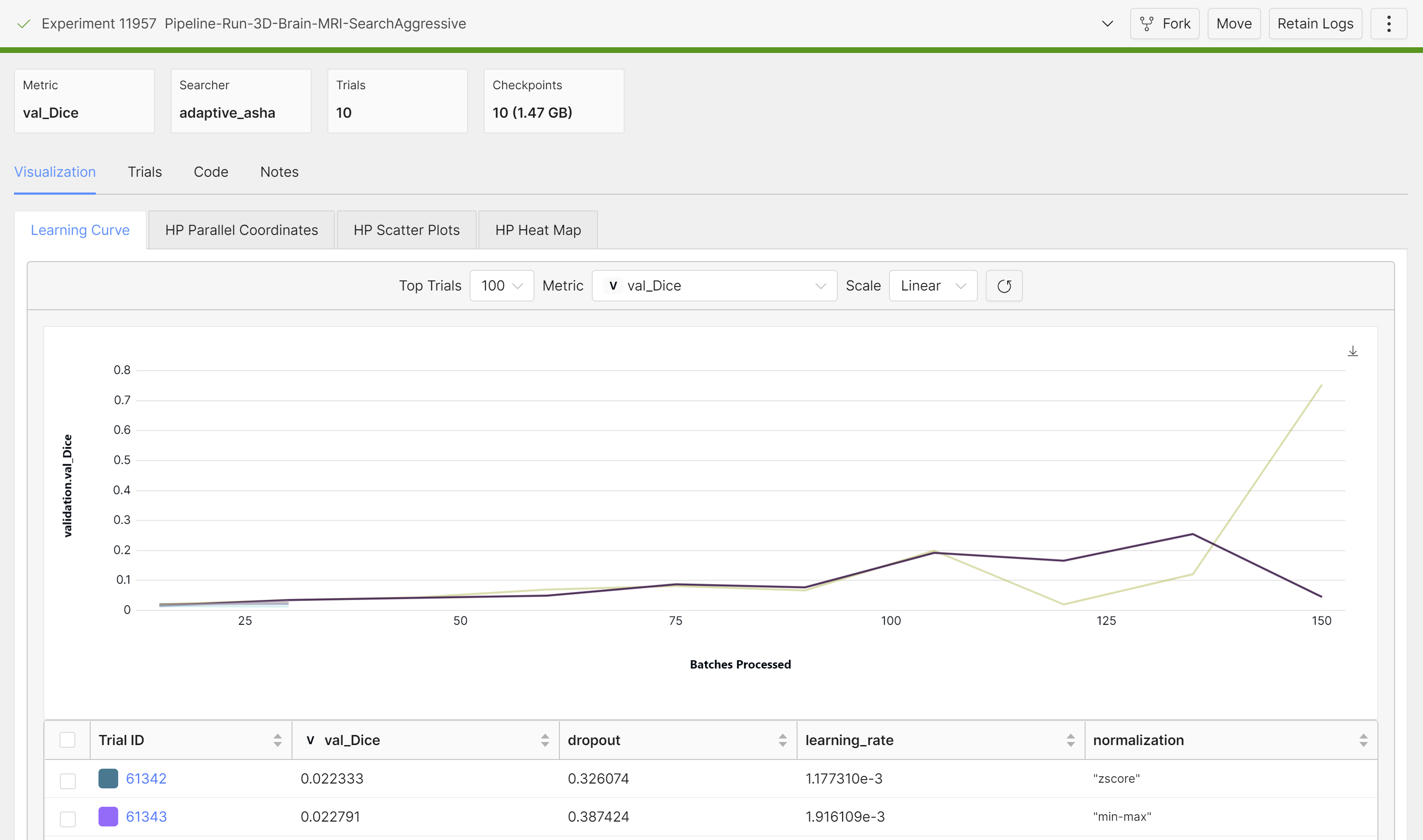
These are from running an aggressive hyperparameter search:

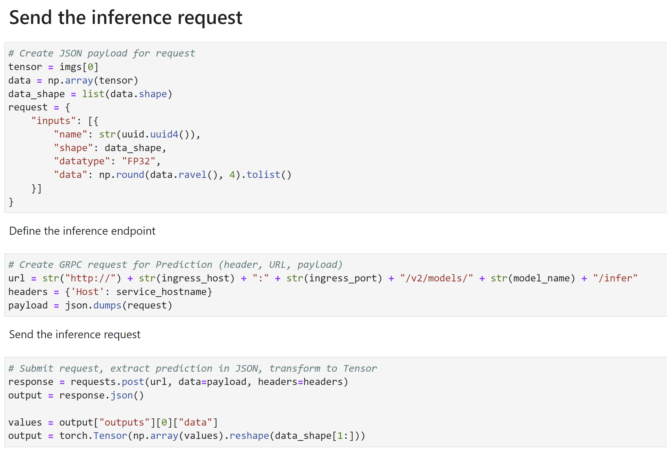
Serving

Once the model is trained, you can also deploy it as an endpoint. Then you can submit inference requests (volumes) and get an output mask:

More on this in the demo video.

Fun fact: If you don’t like Jupyter Notebooks, you can do all of what we covered in this blog using Pachyderm pipelines:

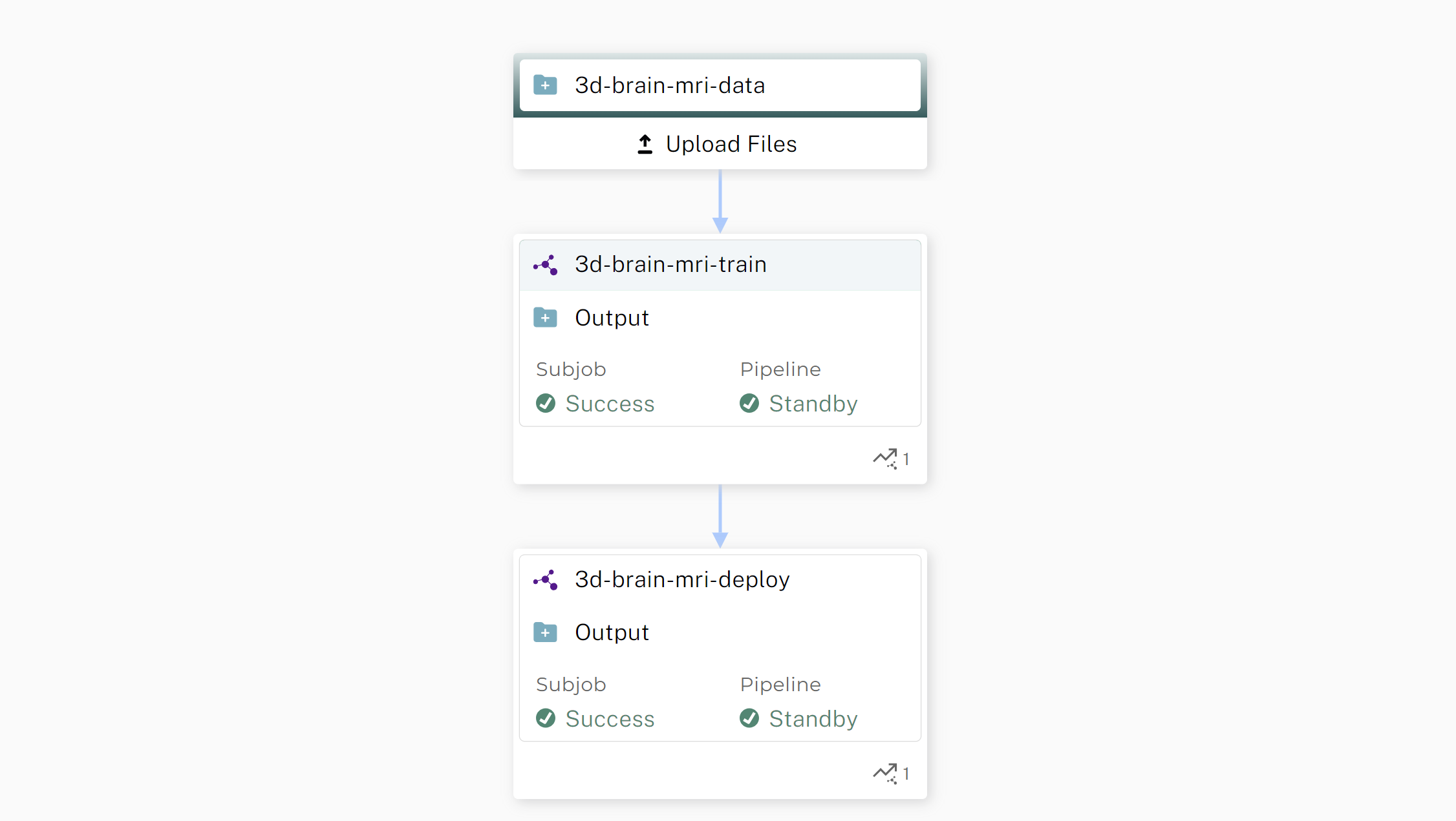
What is a Pachyderm Pipeline?

Each cell in the figure is called a pipeline, and each pipeline has an input and an output. The processing steps in each pipeline can be defined to be whatever you want – all the data preprocessing and finetuning steps we already talked about is defined in the pipeline specification for in 3d-brain-mri-train, for example. The input to the 3d-brain-mri-train pipeline is the raw data, and the output is a model checkpoint. All pipeline steps are fully versioned with a git-like structure, and can be re-run as an end-to-end pipeline to retrain the model on new or updated data, eliminating the need to manually go through data preparation and model training steps. Read more about pipelines in the Pachyderm docs.

Takeaways

3D structural segmentation is a well known problem in radiology. This demo is representative of one of many structural segmentation tasks across different types of data: X-ray, CT scan, and more.

Many times, a model trained at hospital A won’t work on data from hospital B. Even when adjusting for the same MRI acquisition parameters, the same MRI scanners can produce different volumes that can affect the ability of a model to generalize. Different institutions also have different annotation practices, which can further affect model performance.

Having this demo blueprint for institutions to efficiently train their own models on existing infrastructure helps curb some of these issues. Plus, 3D segmentation models are very data efficient. Having 50-100 volumes can often be enough to achieve high segmentation Dice accuracies.

And as a bonus, Determined’s JupyterLab environment and Pachyderm’s data tools make it easier to host and format data, train models, and keep track of them.

If you’re interested in experimenting with this demo yourself, it’s publicly available on GitHub!

Also, check out the demo video where Alejandro walks through the code in more detail.

Stay up to date

Stay up to date by joining our Slack Community!