RuntimeError: CUDA error: out of memory

The worst! GPU memory is a precious resource and running out of it – which produces the PyTorch error above – is a depressingly familiar headache that wastes time and money. Understanding the memory budget for model training is therefore crucial.

In this series of blog posts, we will discuss the most complex component of the memory budget: activation memory. In this first post, we will discuss what it is, what makes it different from other forms of memory, and when it matters. Future posts in this series will dive into more technical details, and demonstrate how to model and measure activation memory costs in PyTorch.

Where It Comes From

What is activation memory? Activation memory comes from the cost of any tensors (“activations”) which need to be saved to perform the backward pass during training. It is a training-only concern: these activations do not need to be saved during inference.

Of course, activation memory isn’t the only contributor to the GPU memory budget. The other major contributors are the model parameters, optimizer state, and gradients.

However, unlike these components, whose memory usage can be calculated simply from the number of model parameters, activation memory depends both on the details of the model architecture, and the properties of the model inputs.

To understand the difference, let’s consider a basic transformer block like in the figure below. If there are \(N\) total parameters in this block, then the memory (in bytes) used by this block’s parameters, optimizer state, and gradients is:

That’s pretty straightforward! Note that these equations assume:

• The optimizer saves two states per model parameter, as done in Adam.
• float32 precision is used everywhere, which means every number uses 4 bytes of memory. Mixed-precision considerations are discussed towards the end of this post.

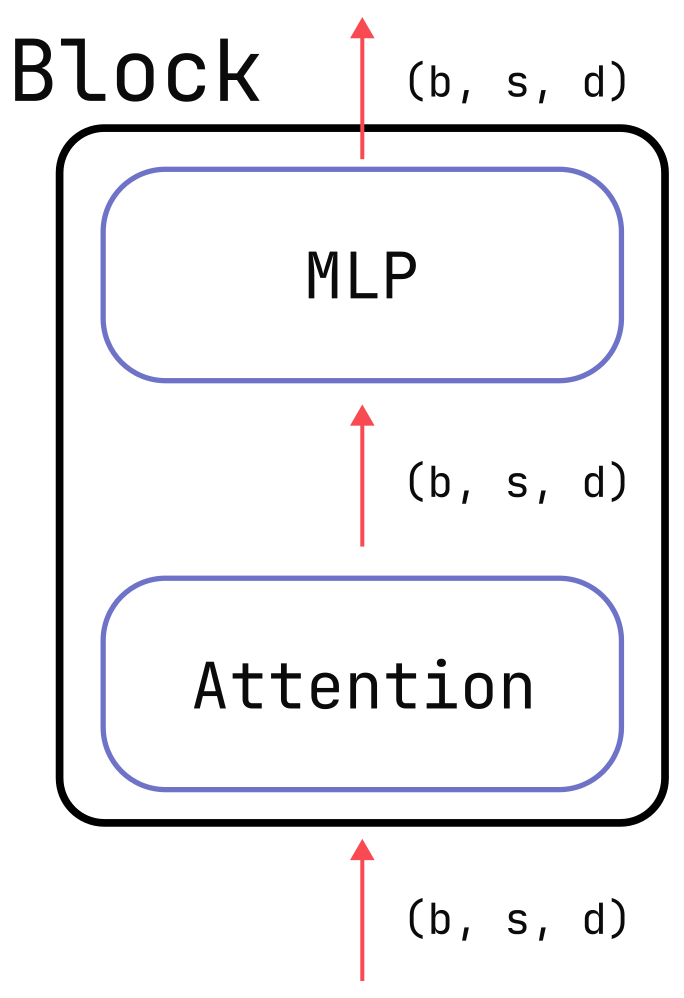
Now let’s consider the activation memory for the same transformer block. Activation memory depends on multiple factors:

• The batch size, \(b\).

• The input’s sequence length, \(s\).

• The activation function used in the MLP layer.

• Whether or not flash attention is used.

Furthermore, many intermediate tensors are generated during the forward pass, but only some have to be saved for the backward pass.

Ultimately, the activation memory for a single transformer block is:

Here, \(d_{m}\) is the size of the model’s hidden dimension, \(n_{h}\) is the number of attention heads, and \(\alpha\) and \(\beta\) are numbers that depend on architectural details.

The two terms in the equation scale differently with the sequence length, \(s\):

• The first term is linear in \(s\). It is derived from the shapes of intermediate tensors:

  • \((b, s, d_{m})\) or \((b, s, 4d_{m})\) in the typical MLP layer.
  • \((b, s, n_{h}, d_{h})\) in the typical attention layer, where \(d_{h} = d_{m} / n_{h}\).

  All of these shapes have a number of elements proportional to \(b\, d_{m}s\), so the \(\alpha\,b\, d_{m}s\,\) term just sums up the corresponding bytes from all of these tensors.

• The second term is (concerningly) quadratic in \(s\) and comes from creating the \((b, n_h, s, s)\)-shaped self-attention scores.

What are the values of \(\alpha\) and \(\beta\)? Is it possible that \(\beta\) is so small that we don’t have to worry about the quadratic nature of the second term? The answer depends on the model architecture and implementation choices. For example:

• For a vanilla transformer block, \(\alpha = 34\) and \(\beta = 5\), so the second term is significant. The derivation for this can be found in the paper, Reducing Activation Recomputation in Large Transformer Models. (These numbers should be regarded as approximate and we will refine their values in a subsequent post.)
• When using flash attention, \(\beta = 0\), so the second term disappears entirely. This, along with increased throughput, are the major advantages of flash attention. Use flash attention, or PyTorch’s scaled_dot_product_attention equivalent, whenever possible.

When It Matters

So, how important is activation memory? It depends!

Let’s consider the ratio of activation memory to non-activation memory costs. As we showed earlier, the non-activation memory costs are all proportional to \(N\), the number of parameters in the transformer block. For a typical transformer block, the value of \(N\) is dominated by the large matrices in the sub-layers whose dimensions are all proportional to \(d_{m}\). If you work through the math, it turns out that \(N \approx 12 d_{m} ^ 2\) (see Section 2.1 of Scaling Laws for Neural Language Models for the derivation). In turn, this means that the sum of the non-activation memory costs per block due to parameters, optimizer, and gradients is:

Assuming we use a flash-attention-like algorithm, so that \(\beta=0\) and \(\alpha=34\), the ratio becomes:

Thus, the higher the number of tokens in the batch (\(b\, s\)) relative to the hidden dimension of the model (\(d_{m}\)), the greater the importance of the activation memory. And this ratio can vary significantly depending on the model:

• For LLama2 7B, \(\texttt{ratio} \approx 0.2b\). Activation memory is similar to other memory costs at typical batch sizes.

• For Megatron-Turing NLG 530B, \(\texttt{ratio} \approx 0.02b\) (pretending we could run this huge model on a single GPU). Activation memory is not a top concern for typical batch sizes.

• For the 7B model trained on million-length sequences, \(\texttt{ratio} \approx 50b\). Activation memory is enormous and completely dominant. Training is not even possible without a specialized algorithm such as RingAttention, as used in this paper.

Given the recent trend of increasingly long sequence lengths, one should expect the importance of activation memory to continually increase in the near future.

Other Considerations

The above analysis was restricted to only the simplest of scenarios: single-GPU training of a full-precision model in which all weights are updated and where only the transformer blocks needs to be accounted for. In this final section, we briefly cover some more advanced topics.

The Language Model Head and Small Models

The above analysis entirely ignored the language-model head. This is a fine approximation for larger models with many layers, but can be very poor for small ones. Small models typically retain large vocabulary sizes (relative to the hidden model size \(d_{m}\)) and the language-model head produces activations with a vocabulary-sized dimension. In small models, this contribution can represent a significant fraction of the overall activation memory. If you see relatively large memory spikes near the end of your forward pass, this is a likely culprit.

Parallelism and Checkpointing

A large model cannot be trained on a single GPU. Instead, the model must be split across multiple GPUs and the specific parallelism strategy affects how much activation memory is generated. Methods such as Tensor Parallelism, Pipeline Parallelism, DeepSpeed ZeRO, Fully Sharded Data Parallel, and Ring Attention all affect the memory costs from activations and other sources in different ways. Another popular strategy is activation checkpointing, which trades memory for compute, by re-calculating activations on demand instead of caching them.

Mixed Precision

Almost all model training actually happens in mixed-precision in which various parts of the forward pass are computed in a lower precision, such as bfloat16. Perhaps unintuitively, this actually increases the contribution of model parameters to the overall memory budget because mixed-precision implementations typically keep both a high-precision and a low-precision copy of the model weights around (for numerical reasons). Nevertheless, mixed-precision can reduce activation memory, since intermediate tensors are often generated in low-precision. Whether or not there’s an overall memory advantage depends on the details, but typically it is indeed a savings.

Parameter Efficient Fine Tuning

There exist many effective training strategies, such as LoRA, which only update a small proportion of the model’s parameters. Such strategies cut the optimizer state memory to a negligible amount, but the activation (and gradient) memory costs can be just as large as they are for full-model training. The specifics again depend on details such as where the to-be-trained weights live inside the model.

What Next?

This was only an introduction to activation memory: what it is and how to perform back-of-the-envelope calculations to reason about it. In the next post, we will dive into the more technical details, including how to measure activation memory directly in PyTorch.