In our last post on LLM finetuning, we showed how to finetune the TinyLlama-1.1B model on a text-to-SQL task using Determined and Hugging Face Trainer.

In this post, we’re going to build on that work and finetune a much larger model, Mistral-7B, for the same text-to-SQL task with the goal of getting better results, particularly on the most challenging examples.

If you recall from the previous blog post, to finetune TinyLlama-1.1B, we used a simple data parallel technique where each GPU keeps a replica of the model and processes batches of data independently. This approach works when the model can fit within a single GPU. However, the memory required to train Mistral-7B exceeds the capacity of an Nvidia A100 GPU with 80 GB of memory! To solve this problem, we will look into two different approaches: LoRA and DeepSpeed, which will allow you to scale up or down the GPU requirements.

Since we stepped through the LLM finetuning code in detail in our last post, here, we’ll only highlight the most critical new code snippets. If you’d like to jump into the code yourself, you can view and download the full example from GitHub.

Here’s what we’ll cover in this post:

• What is LoRA?
• Adding LoRA to the script
• What is DeepSpeed?
• Adding DeepSpeed to the script
• Padding, truncation, and max_length
• Chat formatting
• Training
• Results

What is LoRA?

LoRA (Low-Rank Adaptation) is a parameter-efficient fine-tuning method, meaning that it reduces the number of parameters that need to be trained, thus reducing the amount of GPU memory required.

When fine-tuning an LLM, the goal is to adapt its pre-trained weights to perform well on specific tasks. Let \(W\) represent one of those weight matrices. Traditionally, fine-tuning involves updating all elements of \(W\) directly through gradient descent to reduce task-specific loss. It is easy to see how this process can quickly become expensive with increasing model size.

LoRA introduces a clever approach to address this problem. The main idea stems from the observation that the difference between pre-trained weights and finetuned weights has a “low intrinsic rank”. In plain English, it essentially means that significantly fewer parameters are needed to capture model updates during finetuning.

In more mathematical terms, let \(\Delta W\) be a matrix of size \(d \times k\) that represents the difference between the pre-trained and finetuned weights. If \(\Delta W\) has a low intrinsic dimension, it can be approximated as a product of two smaller matrices \(A\) and \(B\), \(\Delta W = BA\). Here, \(A\) has dimensions \(r\times k\), and \(B\) is \(d\times r\), where \(r\) is an arbitrary value we set.

As long as we set \(r\) to something much smaller than \(d\) and \(k\), we’ll have significantly fewer parameters to update. For example, if \(d\) and \(k\) are both 1000, then computing \(\Delta W\) requires computing gradients for 1 million parameters. With LoRA and \(r = 10\), the number of parameters is \(1000 \times 10\) + \(10 \times 1000\), which is 20000, or just 2% of the original parameter count.

During training, LoRA finetunes the model by focusing on these two smaller matrices, \(A\) and \(B\), rather than updating the whole weight matrix \(W\). By updating \(A\) and \(B\), which hold far fewer parameters between them than \(W\), LoRA captures the gist of the model’s adaptation in a more manageable, less resource-hungry manner. After training, the \(BA\) matrix is added to the original pretrained weights to obtain the new \(W\), thus resulting in the exact same inference cost as in the original model.

Adding LoRA to the script

First install peft, which stands for “parameter efficient fine tuning”:

pip install peft

Initialize the LLM like we did in the previous blog post, but this time use Mistral-7B:

import torch
from transformers import AutoModelForCausalLM

model_name = "mistralai/Mistral-7B-Instruct-v0.2"
model = AutoModelForCausalLM.from_pretrained(
    model_name,
    torch_dtype=torch.bfloat16,
)

Next, create LoraConfig and pass the model into get_peft_model to get the LoRA-fied model:

from peft import LoraConfig, get_peft_model

# This if statement will allow us to turn LoRA on and off.
# hparams holds our configuration options.
if hparams["lora"]:
    peft_config = LoraConfig(
        task_type="CAUSAL_LM",
        inference_mode=False,
        r=8,
        lora_alpha=32,
        lora_dropout=0.1,
    )

    model = get_peft_model(model, peft_config)

The LoraConfig parameters are:

• r: this is the inner dimension of the \(B\) and \(A\) matrices.
• lora_alpha: \(BA\) gets scaled by \(\frac{\alpha}{r}\)
• lora_dropout: The probability of dropping (zeroing out) parameters from the LoRA matrices during training.

What is DeepSpeed?

DeepSpeed is a library that trains models in a memory-efficient way, allowing people to train much larger models on their GPUs than they would otherwise be able to. The simplest way to do distributed training is to make each GPU hold a copy of all parameters, gradients, and optimizer states. DeepSpeed saves memory by making each GPU hold just a slice of each of these, as shown in this figure from the DeepSpeed white paper:

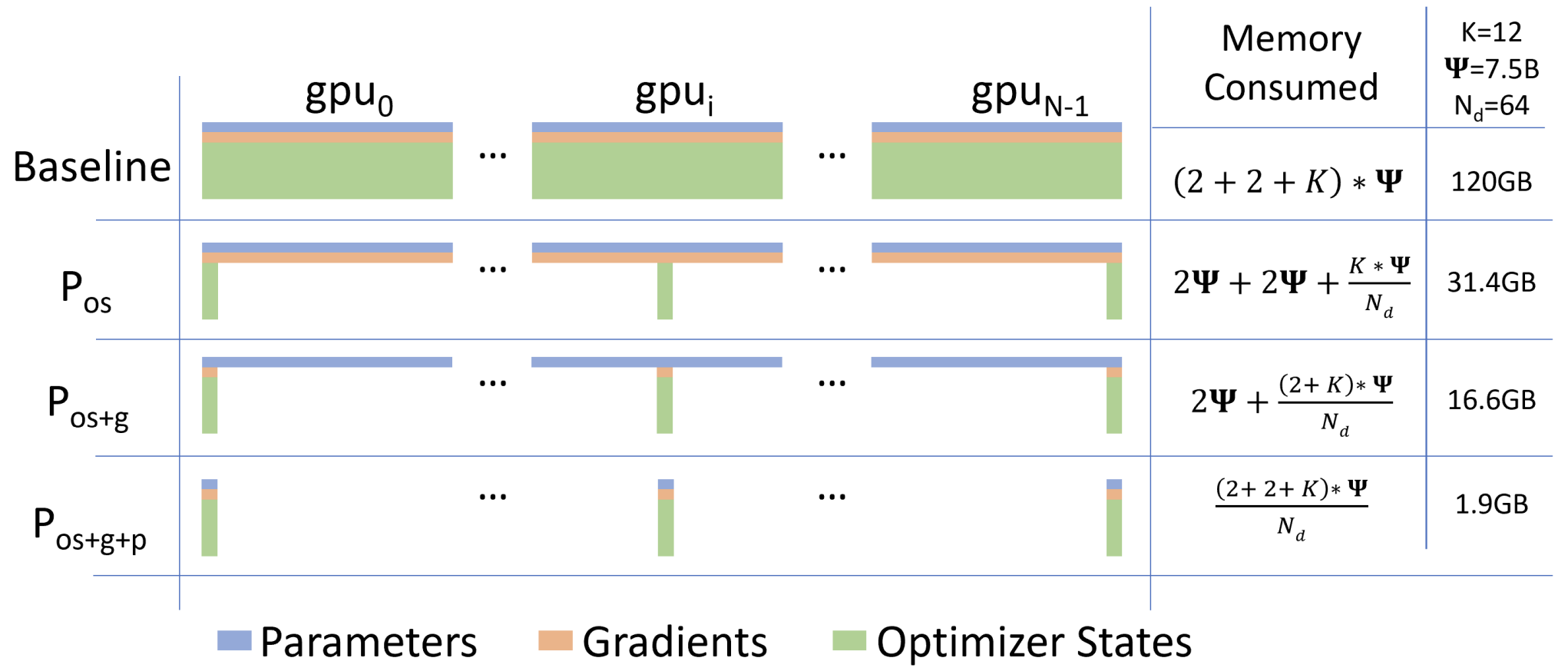
In the figure above:

1. \(P_{os}\) splits optimizer state.
2. \(P_{os+g}\) splits optimizer state and gradients.
3. \(P_{os+g+p}\) splits optimizer state, gradients, and model parameters.

In DeepSpeed these are called “stages”. We’ll use DeepSpeed Stage 3, which is the method with the most memory savings (\(P_{os+g+p}\)). However, even with these memory savings, using DeepSpeed to finetune the full model will still require more memory than using LoRA to finetune the \(BA\) approximation.

Adding DeepSpeed to the script

First install deepspeed:

pip install deepspeed

Then create a JSON file that specifies the DeepSpeed configuration. Don’t be intimidated by its content! You can learn more about it by reading the DeepSpeed docs; however, the code snippet below gives you a solid starting point that should also work for other experiments you may want to run.

Some important options are:

• zero_optimization.stage: the level of memory optimization. Stage 3 provides the most memory savings as described above and in the DeepSpeed documentation.
• scheduler.type: the optimizer’s learning rate scheduler. We’re using WarmupDecayLR.

{
  "fp16": {
    "enabled": "auto",
    "loss_scale": 0,
    "loss_scale_window": 1000,
    "initial_scale_power": 16,
    "hysteresis": 2,
    "min_loss_scale": 1
  },
  "bf16": {
    "enabled": "auto"
  },
  "optimizer": {
    "type": "AdamW",
    "params": {
      "lr": "auto",
      "betas": "auto",
      "eps": "auto",
      "weight_decay": "auto"
    }
  },
  "scheduler": {
    "type": "WarmupDecayLR",
    "params": {
      "warmup_min_lr": "auto",
      "warmup_max_lr": "auto",
      "warmup_num_steps": "auto",
      "total_num_steps": "auto"
    }
  },
  "zero_optimization": {
    "stage": 3,
    "overlap_comm": true,
    "contiguous_gradients": true,
    "sub_group_size": 1e9,
    "reduce_bucket_size": "auto",
    "stage3_prefetch_bucket_size": "auto",
    "stage3_param_persistence_threshold": "auto",
    "stage3_max_live_parameters": 1e9,
    "stage3_max_reuse_distance": 1e9,
    "stage3_gather_16bit_weights_on_model_save": true
  },
  "gradient_accumulation_steps": "auto",
  "gradient_clipping": "auto",
  "train_batch_size": "auto",
  "train_micro_batch_size_per_gpu": "auto"
}

Using this config file is as simple as passing the config’s filepath to TrainingArguments as deepspeed. Since we’re using Determined to manage our experiments, we’ll add the deepspeed flag to the training_args section of the yaml config file:

hyperparameters:
  training_args:
    deepspeed: "ds_configs/ds_config_stage_3.json"

Padding, truncation, and max_length

When processing batches of samples, the tokenizer pads the shorter samples so that they have the same length as the longest sample. Hence, one way to reduce memory requirements is to truncate the longest samples in the dataset. But we have to be careful:

• If we truncate the left side of each sample, we’ll be removing part of the instructions and prompt, which would make it difficult for the LLM to answer well.
• If we truncate the right side of each sample, we’ll be removing part of the “answer”, which would make it difficult for the LLM to learn how to fully answer the user’s prompt.

For example, let’s see what happens when we truncate a training sample down to 100 tokens. Here’s the full sample:

[INST] You are a helpful programmer assistant that excels at SQL. 
When prompted with a task and a definition of an SQL table, 
you respond with a SQL query to retrieve information from the table. 
Don't explain your reasoning, only provide the SQL query.
Task: how many tracks have their producer as mike punch harper ?
SQL table: CREATE TABLE table_203_353 (
    id number,
    "#" number,
    "title" text,
    "producer(s)" text,
    "featured guest(s)" text,
    "time" text
)
SQL query:  [/INST]
SELECT COUNT("title") 
FROM table_203_353 
WHERE "producer(s)" = 'mike "punch" harper'

Here’s the same sample with left-side truncation:

203_353 (
    id number,
    "#" number,
    "title" text,
    "producer(s)" text,
    "featured guest(s)" text,
    "time" text
)
SQL query:  [/INST]
SELECT COUNT("title") 
FROM table_203_353 
WHERE "producer(s)" = 'mike "punch" harper'

And here’s the same sample with right-side truncation:

[INST] You are a helpful programmer assistant that excels at SQL. 
When prompted with a task and a definition of an SQL table, 
you respond with a SQL query to retrieve information from the table. 
Don't explain your reasoning, only provide the SQL query.
Task: how many tracks have their producer as mike punch harper ?
SQL table: CREATE TABLE table_203_353 (
    id number,
    "#

As you can see, truncation can remove a lot of important information. Ideally, we want to truncate only the outlier samples (the really long ones) so that most training samples are unaffected. Let’s look at the distribution of sample lengths for the hard dataset’s training split:

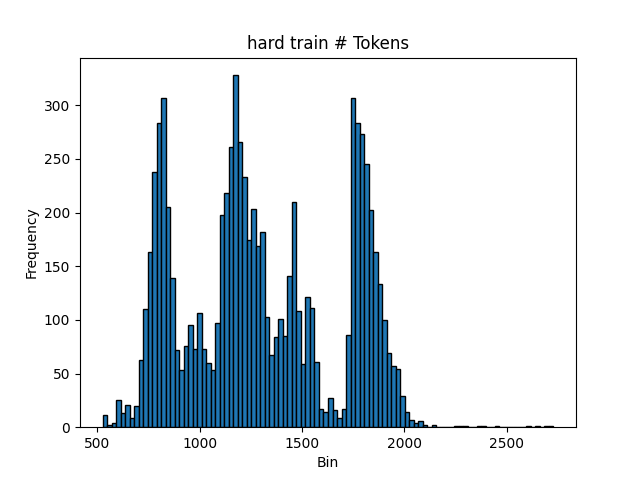
It looks like most samples have fewer than 2000 tokens (let’s say 2048 for a nice power-of-2 number). Therefore, for each batch of samples we will:

• Truncate them from the right so that they are at most 2048 tokens long. Samples shorter than 2048 tokens won’t be truncated at all.
• Add padding tokens to the right side of samples so that they all have the same length as the longest sample.

To accomplish this, we set the padding and truncation side when we initialize the tokenizer:

tokenizer = AutoTokenizer.from_pretrained(
      model_name,
      padding_side="right",
      truncation_side="right",
  )

Then specify the truncation length when tokenizing a sample:

tokenized = tokenizer(sample, padding=True, truncation=True, max_length=2048)

With this setting, we truncate only 24 of the hard dataset’s training set samples, which means most of the training set is left intact.

As a sanity check, let’s look at the sample length histogram with padding and truncation enabled, and a batch size of 4:

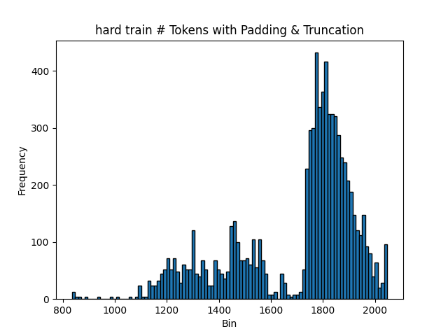
In this histogram, the largest bin size is around 2000. Compared to the previous histogram, the distribution has shifted to the right due to padding.

Chat formatting

The TinyLlama model required us to define the chat template due to a discrepancy between the expected template and the default tokenizer’s template.

Luckily, Mistral’s tokenizer has the correct template, so we can just use tokenizer.apply_chat_template without defining the template ourselves. This function expects a list of strings and their roles (like “user” or “assistant”). Unlike TinyLlama, Mistral’s chat template does not accept a “system” role, so we’ll prepend the user prompt with our system prompt:

def get_chat_format(element, model_name):
    system_prompt = (
        "You are a helpful programmer assistant that excels at SQL. "
        "When prompted with a task and a definition of an SQL table, you "
        "respond with a SQL query to retrieve information from the table. "
        "Don't explain your reasoning, only provide the SQL query."
    )

    user_prompt = "{system_prompt}\nTask: {instruction}\nSQL table: {input}\nSQL query: "

    return [
        {"role": "user", "content": user_prompt.format_map(element)},
        {"role": "assistant", "content": element["response"]}
    ]

# We apply this function to every dataset sample
formatted = tokenizer.apply_chat_template(
    get_chat_format(element, model_name), tokenize=False
)

Training

Now we’re ready to train the model. As we did in our last post, we’ll use Determined for experiment tracking and resource provisioning. First, we need to install Determined:

pip install determined

Then, we need to make a small change to our training script so that the correct distributed context is used for DeepSpeed:

+    if training_args.deepspeed:
+        distributed = det.core.DistributedContext.from_deepspeed()
+    else:
+        distributed = det.core.DistributedContext.from_torch_distributed()

    with det.core.init(distributed=distributed) as core_context:
        det_callback = DetCallback(
            core_context,
            training_args,
        )
        main(training_args, det_callback, hparams)

We create two Determined yaml configuration files: one for LoRA and one for DeepSpeed.

To finetune with LoRA:

det e create lora.yaml .

To finetune with DeepSpeed:

det e create deepspeed.yaml .

Results

Mistral Performance

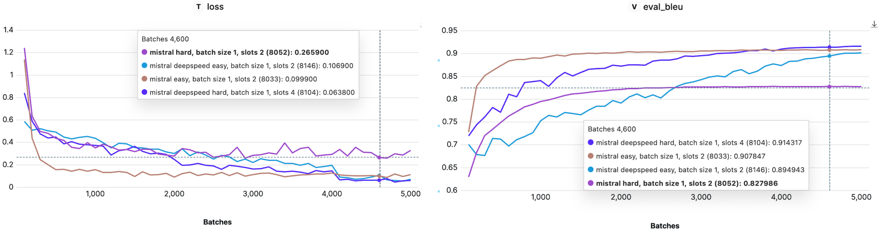
Let’s first examine how LoRA compares to full-parameter fine-tuning in terms of model performance. Remember, the ability to do a full-parameter fine-tuning of Mistral-7B is enabled by the DeepSpeed library, which effectively distributes the model across multiple GPUs. In the chart below, we show the BLEU score on the evaluation dataset for each dataset difficulty.

For the simplest datasets, LoRA and DeepSpeed exhibit similar performance levels. However, as complexity increases, so does the performance divergence, with full-parameter fine-tuning taking the lead. The increasing performance gap stems from the fact that LoRA operates on an approximation of model weights instead of using the weights directly, which essentially means it trains with fewer parameters. Effectively, LoRA’s constrained parameter set may not capture certain patterns in the data. Hence, more complicated tasks are more likely to experience a drop in performance when compared to full-parameter fine-tuning.

We can also see the effect of LoRA’s approximation in the loss and BLEU scores during training. For the hard dataset, Mistral trained with DeepSpeed (full-parameter fine-tuning) continuously decreases the training loss and improves the BLEU score. On the other hand, when the model is trained with LoRA, we can see that the training loss saturates at some level, indicating we reached the limit of what it can learn with the current approximation.

Note that the approximation level depends on the value of \(r\) set in the LoraConfig - the lower \(r\) is, the smaller \(A\) and \(B\) become, and the stronger the approximation is. Hence, if you consider LoRA for your task, selecting the right \(r\) can help you find the balance between approximation and model performance.

TinyLlama Performance

How does full-parameter fine-tuning compare with LoRA, when using a smaller model? Before scrolling down, try to answer this question for yourself! To answer this question empirically, we ran TinyLlama-1.1B with LoRA and compared the results to the full-parameter fine-tuning we did in the previous blog post.

In contrast with the results we got for Mistral, TinyLlama trained with full-parameter fine-tuning outperforms LoRA across all three tasks, by a large margin. One explanation for this is that TinyLlama is already a fairly small model, and using LoRA reduces the parameter count even further, such that there aren’t enough parameters to learn effectively.

Training time

While LoRA reduces the number of trainable parameters, making the backward call faster and the memory footprint lower, it also introduces new parameters (\(A\) and \(B\)) and additional operations to the model. In the chart below, we show the comparison of training times between TinyLlama and Mistral when trained with or without LoRA. As expected, we observe that using LoRA in general leads to faster training, with the difference proportional to the model size and \(r\).

Takeaways: TinyLLama vs Mistral

Choosing between TinyLlama and Mistral — and whether to use LoRA or full-parameter fine-tuning—really depends on what we’re trying to do. If the task isn’t too complex, TinyLlama with full-parameter fine-tuning is quick and gives great results. However, for more challenging tasks, stepping up to Mistral might be the way to go. Here, LoRA can help make fine-tuning more manageable, cost-wise, without sacrificing too much on performance.

Summary

In this blog post, we fine-tuned Mistral-7B on a text-to-SQL dataset using LoRA and DeepSpeed. While both approaches enable us to run models exceeding the memory capacity of a single GPU, they offer different solutions to the problem. LoRA reduces the number of parameters to train via approximation, whereas DeepSpeed enables training of all model parameters by distributing the model across multiple GPUs. As we have observed, both approaches come with certain trade-offs. For simple tasks, full-parameter fine-tuning on a smaller model may suffice. On the other hand, for complex tasks, leveraging larger models will be necessary, and the choice between LoRA and full-parameter fine-tuning with DeepSpeed depends on the available compute resources.

Want to run the code?

View and clone the full example from GitHub.

If you have any questions, feel free to start a discussion in our GitHub repo and join our Slack Community!